At a drug discovery CRO I ran ADME assays on an Agilent 1100 quaternary pump with an MSD. The method was a 15 minute gradient. That was fine until the chemistry team started making more compounds. More compounds meant more assays, and more assays meant more samples than a 15 minute method could clear in a day.
So I set out to make the method shorter. I had come from a bioanalytical CRO where I ran 2 and 3 minute gradients, so I knew what a fast method looked like, and I did what had worked there. Shorter column, 100 mm down to 50 mm, and narrower, 4.6 mm down to 2.6 mm.
The 2.6 mm was deliberate. The obvious choice was 2.1 mm, but the 1100 tops out at 400 bar, and the narrower the column the more backpressure it costs at the same flow. 2.6 mm was the compromise: narrow enough to cut the volume, wide enough to stay inside what the instrument could push. On paper that should have given me 3 to 4 minutes.
It did not. At 4 to 5 minutes I had carryover. I shortened the column and the method still would not go as fast as the one I had run before on the same kind of chemistry.
It took me half a day to work out why, and I got there sideways. I ran isocratic injections and watched how long it took to get reproducible peaks with nothing carried over from the one before. The thing I was fighting was the internal volume of the 1100, and the part of it that decides how short a gradient can be is the dwell volume. The UPLC I had used before had a fraction of it.
I never measured it. I inferred it, which is why it took half a day instead of half an hour.
What dwell volume is
Dwell volume is the volume between the point where the solvents are mixed and the head of the column. It is also called the gradient delay volume.
When you program a gradient to start at time zero, the pump starts changing the composition at time zero. The column does not see that change until the new composition has been pushed all the way through the mixer, the tubing, and the injector flow path. Until then the column is still running the starting composition.
So the gradient is late. How late depends on the flow rate:
dwell time = dwell volume / flow rateAt 1 mL/min, a 1,100 µL dwell volume means the gradient reaches the column 1.1 minutes after the method says it starts.
None of this matters for an isocratic method. The composition is not changing, so a delay in changing it costs nothing. Dwell volume is a gradient problem.
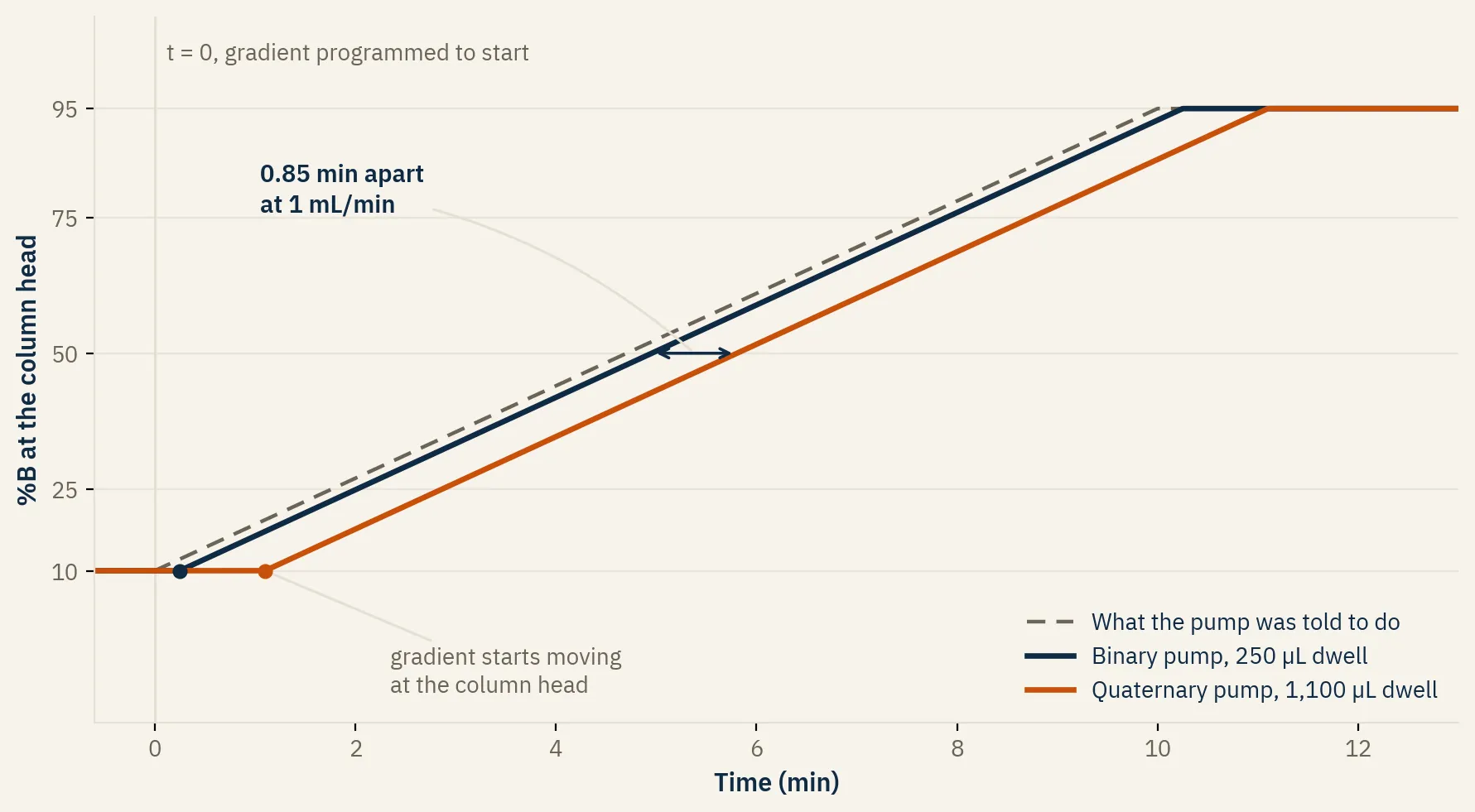
The same gradient, programmed identically on two systems. The binary pump delivers it 0.25 minutes late, the quaternary 1.1 minutes late. Nothing about the method changed. Only the volume it had to travel through before reaching the column.
Why the number is different on every system
Dwell volume is not a specification anyone quotes at you. It is a consequence of how the pump mixes.
Low-pressure mixing (usually a quaternary pump) blends the solvents through a proportioning valve before the pump. So the mixed solvent has to travel through the pump heads, the damper, the mixer and all the tubing before it reaches the column. Everything in that path counts.
High-pressure mixing (usually a binary pump) runs two pumps, one per solvent, and combines them after the pumps at high pressure. The mixed solvent only has to cross the mixer and the tubing. Much less volume.
| System type | Mixing | Typical dwell volume | Delay at 1 mL/min |
|---|---|---|---|
| Quaternary, low-pressure mixing | before the pump | 600 to 1,500 µL | 0.6 to 1.5 min |
| Binary, high-pressure mixing | after the pumps | 100 to 400 µL | 0.1 to 0.4 min |
| UHPLC, high-pressure mixing | after the pumps | 100 to 200 µL | 0.1 to 0.2 min |
These are typical ranges, not values you can assume. Two instruments of the same model can differ. The mixer can be swapped, and the tubing between the injector and the column is whatever somebody cut last time.
What it does to a chromatogram
The whole gradient shifts later by the dwell time. That part is easy to picture and it is the smaller half of the problem.
The larger half is that the delay acts as an isocratic hold at the starting composition. For the first 1.1 minutes on that quaternary system, the column is running at the initial %B whether you asked for a hold or not.
Early peaks are the ones that suffer. A compound eluting at 2 minutes spends more than half its run in that unplanned hold, so its retention factor is set by the starting composition rather than by the gradient. Two early peaks will not shift by the same amount, so the selectivity between them changes, and with it the resolution. That is the part that fails a system suitability test. Late peaks barely notice, because by then the gradient has caught up. That is why a transfer usually breaks the early part of the chromatogram and leaves the rest looking fine.
If the method already has an initial hold, the effective hold is the programmed hold plus the dwell time. On a system with a large dwell volume, a 1 minute hold is really a 2.1 minute hold.
It also sets a floor on how fast you can go
Transfer is the usual way people meet dwell volume. Making a method faster is the other way, and it is the one that caught me.
Cycle time is the dwell time, then the gradient, then whatever it takes to flush the system and re-equilibrate the column for the next injection. On a system with a large internal volume all three are longer.
The arithmetic gets unforgiving as the gradient gets shorter. A 1,100 µL dwell volume at 0.5 mL/min is 2.2 minutes of delay. Ask that system for a 3 minute gradient and most of the run is over before the column sees any change in composition. The gradient you designed is not the gradient that runs.
Carryover has its own causes and deserves its own piece, but it travels with this one. A short run does not give the flow path enough time to flush, so what is left from the previous injection turns up in the next. The volume in the system sets that, which is why a shorter column did not fix it for me.
An older quaternary system can run a fast gradient. It cannot run the same fast gradient as a UHPLC with a tenth of the dwell volume, and no column change will close that gap.
One more thing about that 1100, separate from the story above but learned on the same instrument. It leaked, at the column fittings and at the pump outlet, whenever a column change pushed the backpressure up. Narrow bore did it. So did longer columns. The pressure was still reading below 400 bar each time.
The stated ceiling is what the pump can generate. It is not a promise about every fitting between the pump and the detector, especially on a system that has been in service for years. Check the connections after any change that raises backpressure, and treat a column change as one.
How to measure it, in under half an hour
You do not need a service engineer for this. The test is a gradient with no column and a tracer you can see.
- Take the column out and put a zero dead volume union or a capillary in its place.
- Mobile phase A is water. Mobile phase B is water with about 0.1% v/v acetone.
- Set the detector to 265 nm, where acetone absorbs and water does not.
- Leave the injector in the inject position for the whole run. The loop is part of the flow path your method uses, so it is part of the dwell volume. Measure with it bypassed and you will get a number smaller than the one your method actually sees.
- Run a linear gradient, 0 to 100% B, over 10 to 20 minutes. Use the full range here even though no real method does, because you are measuring the system and not separating anything.
- Watch the baseline ramp.
What you get is not a clean ramp. Dispersion rounds off both corners, so the start and the end of the rise are the least reliable parts of the trace. The middle is the part to trust, and the construction works off it in three steps.
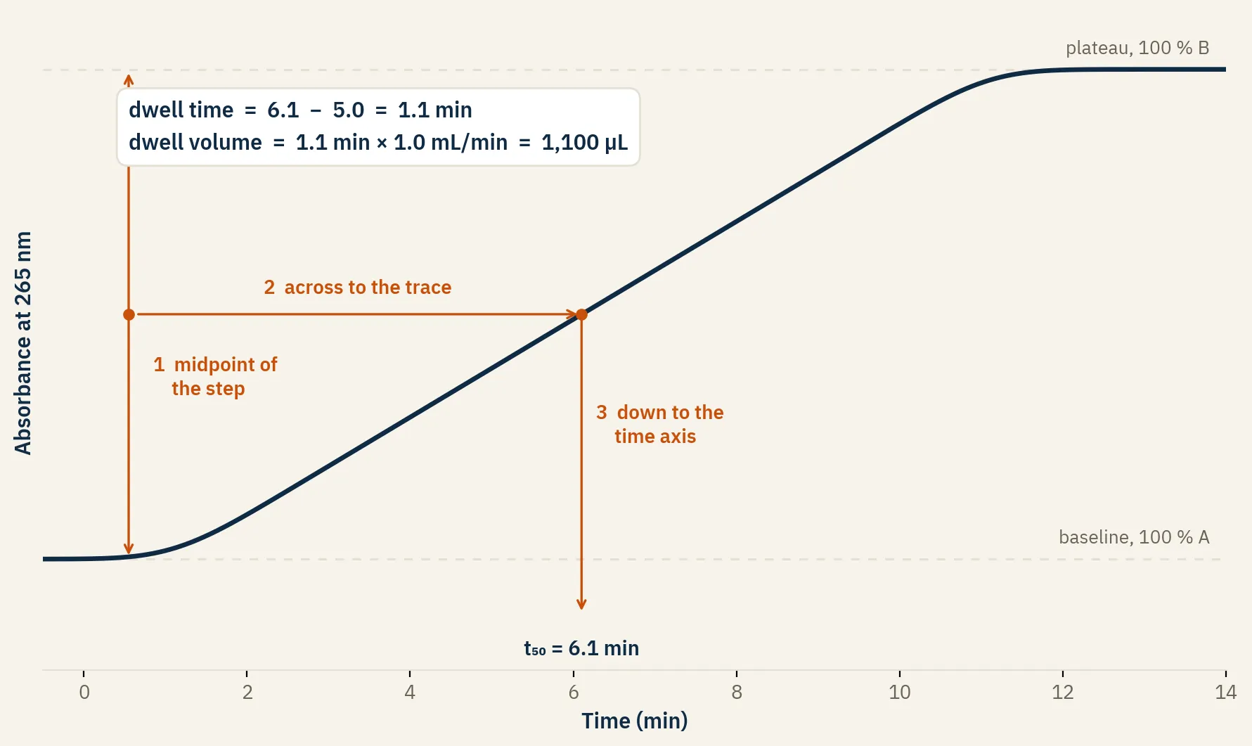
The reliable landmark is the middle of the step, not either end of it.
- Find the midpoint between the low baseline and the high plateau.
- Draw a line across from that midpoint until it meets the rising trace.
- Drop straight down to the time axis. That time is t50.
Then subtract half the gradient time, and multiply by the flow rate:
dwell time   = t50 - (gradient time / 2)
dwell volume = dwell time x flow rate
In the trace above, t50 is 6.1 minutes on a 10 minute gradient, so the dwell time is 1.1 minutes. At 1 mL/min that is 1,100 µL.
There is a second way to read it: extrapolate the straight part of the ramp back down to the starting baseline, and the time where they meet is the dwell time. It gives a similar answer. The midpoint method is easier to do consistently, which matters more when two people are measuring two instruments and comparing.
Do it on both systems. The number you care about is the difference between them, rather than either number on its own.
Two cautions. The flow rate you test at does not matter, because you are measuring a volume and then converting. Pick something convenient: 2 mL/min gets the test over quickly. The plumbing does matter. Swapping in a shorter connecting tube or a different mixer changes the answer, so measure the system in the state the method runs in.
What to do about the difference
flowchart TD
    A[Gradient method moves<br/>to a different system] --> B[Measure dwell volume<br/>on both, acetone test]
    B --> C{New system's dwell<br/>vs the old one}
    C -->|Smaller| D[Add an initial isocratic hold<br/>equal to the difference]
    C -->|Larger| E[Shorten the initial hold<br/>by the difference]
    E --> F{Is there a hold<br/>long enough to shorten?}
    F -->|Yes| G[Adjusted. Re-run the SST]
    F -->|No| H[Delay the injection<br/>by the difference instead]
    D --> G
    H --> G
If the new system has a smaller dwell volume, the gradient arrives too early. Add an isocratic hold at the start equal to the difference, and the column sees the same profile it saw before.
If the new system has a larger dwell volume, the gradient arrives too late. Shorten the initial hold by the difference. If there is no hold to shorten, delay the injection instead: let the gradient start, wait the difference, then inject.
Both are small edits to the gradient table. Neither touches the column, the mobile phase or the sample preparation, which is why finding the cause first matters so much here. A lab that starts by changing the column has already changed two things at once.
If the method is compendial or validated, check what your own change control and the applicable pharmacopoeial rules allow before editing anything. An adjustment for dwell volume is normally allowed. Being allowed to make it does not mean you can make it without writing it down.
Where this shows up first
Usually in system suitability. The resolution of the first critical pair drops below the limit, or a retention time sits outside its window, on a system that is otherwise working perfectly. I have written elsewhere about what an SST failure is actually telling you. This is one of the cleanest examples. The test is doing its job. The instrument is fine, the method is fine, and the two were never matched to each other.
Measure the dwell volume on every gradient system in the lab once. Write the number on a label on the front of the instrument. It takes an afternoon for a whole lab, and it turns a two week transfer problem into a two minute calculation.
The number holds unless somebody changes the plumbing, so re-check it every 6 to 12 months alongside whatever performance evaluation the system already gets. A number that has moved when nothing was supposed to have changed is itself worth knowing about.
I would have found my answer in half an hour with a union and a bottle of acetone. Instead I spent half a day inferring it from isocratic injections, and I still did not have a number at the end of it, only a conclusion.
That conclusion did have an ending. Once it was clear the limit was the instrument rather than the column or the method, the case for different hardware wrote itself. I put the purchase forward, we bought an Agilent 1290, and I was trained on it by the service engineer and did the method development and the transfers. 2.1 mm columns, 2 to 3 minute gradients, on OpenLab CDS. The methods I could not build on the 1100 were straightforward on a system with a fraction of the dwell volume.
The number is what turns that into an argument rather than a preference. “The gradient is late” is an opinion. “The gradient arrives 1.1 minutes late and the assay needs a 3 minute cycle” is a specification, and it is the kind of sentence a purchase gets approved on.
The habit underneath this is one I keep coming back to. I have made the same argument about apparent pKa, which is a different number measured a different way: the value that governs your method is the one measured on your system, not the one someone else measured on theirs.